Category: Economic Policy

I. Introduction

Since the establishment of formal diplomatic relations between the United States (US) and the People’s Republic of China (PRC) in 1979, there has been a rapid growth of bilateral trade. Trade in goods and services between the US and China increased from $15.4 billion in 1979 to $180 billion in 2000, growing at roughly 10% annually. This growth accelerated in 2000 when the US granted China permanent normal trade relations (PNTR), which paved the way for China’s accession to the World Trade Organization (WTO) in 2001. This served as a milestone in China’s “reform and opening” process and signified that the US and the global economic community recognized China as an equal partner. To join the WTO, China agreed to numerous conditions, including expanding market access for foreign firms to sell goods and services directly in Chinese domestic markets, lowering import tariffs, and opening the telecommunication and finance sectors to more foreign competition.

There is no doubt that WTO membership greatly benefitted the Chinese economy; expanded access to foreign markets increased net exports and economic growth as productivity increased due to greater competition. However, many in the US argue that China’s accession has hurt the US economy and workers, pointing to the ever-growing bilateral trade deficit, the loss of US manufacturing jobs and growing unemployment, and stagnating US economic growth as evidence that China has used unfair, if not illegal, trade practices to take advantage of the US. These trade practices allegedly include currency manipulation, government subsidies for land, capital, utilities and tax breaks, intellectual property (IP) theft, and lax environmental and worker health and safety standards. Furthermore, many criticize the WTO for its lax enforcement regarding China’s alleged illegal trade practices. While these trade practices have undoubtedly played a role in the bilateral trade deficit, a closer look reveals that it is only partly responsible for a stagnating US economy. 

II. Background on Chinese Economic Growth

The People’s Republic of China was established in 1949 by the Chinese Communist Party (CCP). During this period, China struggled with unsuccessful socialist economic reforms and internal turmoil within the CCP. In 1978, Deng Xiaoping, a key political player under Chairman Mao, became paramount leader and began the ‘reform and opening’ process intended to jumpstart the Chinese economy and bring the country out of poverty. Deng echoed the sentiment behind these reforms later in 1992 when he stated: 

“After the basic socialist system has been established, it is necessary to fundamentally change the economic structure that has hampered the development of the productive forces and to establish a vigorous socialist economic structure that will promote their development.”

Deng enacted a series of economic policies and reforms, particularly in industry and agriculture, that emphasized individual responsibility and greatly improved productivity. In 1986, China applied for membership in the General Agreement on Tariffs and Trade (GATT, the predecessor organization to the WTO). If granted entry, membership in GATT would greatly expand China’s export market as members would eliminate or reduce import tariffs on Chinese goods, and emphasize China as a destination for foreign direct investment (FDI). 

Though Deng’s economic reforms successfully jumpstarted the Chinese economy, the country still struggled with extreme poverty and poor standard of living. China’s GDP per capita placed the country in the top half of low-income countries. In 1990, two-thirds of China’s population, or roughly 750 million people, were living below the International Poverty Line in extreme poverty, defined by the United Nations as living on less than 1.90 international dollars per day.

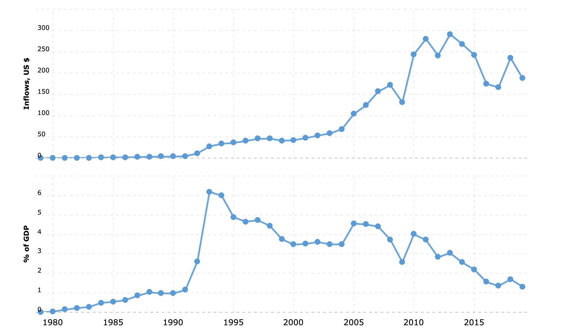
While foreign direct investment (FDI) increased by a factor of 13 between 1980-92 and 1986-88, the growth largely represents its originally low base. Additionally, though FDI inflows into China were large in the early 1990s, by the end of the decade the growth had stagnated. As shown in Figure 1, FDI inflow remained below 2% of gross domestic product (GDP) and below US$12 billion until 1992, mainly due to Chinese restrictions on FDI, government corruption, and inefficient state-owned enterprises (SOEs). FDI inflows did not begin to significantly increase until 2004, peaking at $290.9 in 2013.

Figure 1: FDI Inflow in Total and as Percent of GDP

The share of exports of goods and services in China’s gross domestic product (GDP) steadily increased in the 1980s and 1990s. However, total exports remained low as Chinese businesses had limited access to foreign markets and were subject to high import tariffs. Total exports did not begin to significantly increase until 2002, following WTO accession.

The Asian financial crisis in 1997 particularly affected Thailand, Malaysia, South Korea, and Indonesia. As the value of their currency dropped, there were rapid outflows of FDI and the stock market plunged. During this time, China held its exchange rate steady and provided a great source of stability for the region in addition to offering more than $4 billion in financial aid, a stark contrast to President Bill Clinton who described the Southeast Asian economies as temporarily experiencing a “few glitches in the road.” The crisis revealed the vulnerability of the Chinese economy, which was heavily dependent on cheap exports to fuel its rapid economic development. Since then, the Chinese government has emphasized the need to increase domestic consumption and reduce reliance on exports. 

The US played a major role in China’s negotiations to join the WTO because the two countries had significant bilateral economic and trade interests, and because of US concerns surrounding how China’s exports would impact the international trade hierarchy. Negotiations stalled in June 1989 following the Tiananmen Square massacre and later in 1991 relating to unfair Chinese trade practices including import restrictions that built up net exports while Chinese companies evaded international rules on exports. Throughout the 1990s, China’s Most Favored Nation (MFN) status was increasingly political and tied to human rights concerns.

To join the WTO, China engaged in bilateral negotiations with each interested WTO member to establish market access concessions and commitments in the goods and services area, including tariffs on industrial and agricultural goods and Chinese commitments to open up its market to foreign services suppliers. China also undertook politically and economically risky reforms to uphold free market values of the WTO as a condition for membership. These included: 

• Increasing transparency of trade information and law to both foreign and domestic companies
• Lowering import tariffs on agricultural and industrial products
• Permitting foreign firms to sell directly in Chinese domestic markets
• Opening the telecommunication and finance sectors to more foreign competition

Accession to the WTO triggered and accelerated internal domestic reform. WTO rules served China’s own goal of building a socialist market economy, set in 1992 by Deng, and aided in the transition from a decades-long planned economy to a market-oriented economy. Deng used membership requirements for accession to the WTO as a lever to achieve fundamental changes in SOEs and state-owned banks and overcome bureaucratic obstacles. Whereas Chinese import-exports used to be monopolized by a few dozen SOEs and ministries, after accession hundreds of thousands of Chinese enterprises became involved in import-export. This accelerated the volume of Chinese import-exports and expanded the variety of goods they offered. The central government lessened restrictions which previously constrained the private sector, encouraged private investment in industries that were traditionally dominated by SOEs, and reduced top-down control of Chinese enterprises. Productivity growth post-WTO accession also increased, driven by the entry and exit of firms increasingly allowed due to China’s decentralized reforms. SOEs faced greater accountability for their business decisions and faced the full forces of global competition for the first time, which placed pressure on domestic firms to lower their cost structure to survive. Firms that could not compete were forced to exit the market, increasing overall productivity. 

China also reallocated labor and capital from farms to factories and from inefficient SOEs to more efficient private businesses. With China’s abundant labor supply and relatively scarce supply of arable land and natural resources, manufacturing was the primary beneficiary of reform-induced industrial restructuring. China’s reorientation toward manufacturing was further aided by substantial inflows of foreign direct investment (FDI). China accounts for 75% of all growth in manufacturing value added that has occurred in low- and middle-income economies since 1990. 

Entrance into the WTO provided China with numerous benefits:

• It was an important boost to China’s global leadership as it signaled the US and the global economy recognized China as an equal partner. 
• It strengthened US-China bilateral economic relations, which were strained over the issue of Taiwan and human rights violations. 
• Chinese exports could access new markets through Most Favorable Nation (MFN) status with all members of the WTO, which allows China to face the same trade barriers as competitors. 
• China experienced looser investment restrictions, which led to a growth in Chinese capital.
• China no longer faced the uncertainty of being hit with high tariffs on its exports to the US. This encouraged Chinese firms to invest in paying the fixed costs associated with engaging in international trade and entering the export market.  The US had applied low tariffs on Chinese imports since 1980, but every year Congress met to decide whether to revert to much higher tariff rates that had been assigned to some non-market economies, which averaged 24%.

Read More

• Read more about other conditions for China to join the WTO here. 
• Read China’s White Paper from 2018 that lays out the government’s official position on the US-China trade relationship.
• Read more about the role of state-owned enterprises in China’s economy here. 

III. Impact of Increased Chinese Imports on the US Economy and Employment

A country’s total trade is measured by the sum of its imports (products it buys from other countries) and its exports (products it sells to other countries), both in goods and services. A trade deficit exists when a country’s net exports (calculated by subtracting imports from exports) is negative, meaning the country imports more goods and services than it exports. A trade surplus exists when the opposite occurs. The US has bilateral trade deficits with some trading partners and bilateral trade surpluses with others. Overall, the US had a trade deficit of $678.7 billion in 2020. Bilateral trade deficits typically occur because countries have certain comparative advantages. For example, the US has the comparative advantage in goods and services that require high degrees of human capital and China has the advantage in light manufacturing. 

The US has had a trade imbalance with China since at least 1985 which remained below $85 billion. By 2000, however, the bilateral deficit reached $85 billion and for the first time exceeded the bilateral deficit with Japan. Between 1986 and 2019, the US trade deficit with China grew by 18.4 percent annually. Post-WTO accession, US exports increased as the US gained an export market, but not nearly as much as US imports from China increased. In 2007, US imports with China fell as consumers were hit hard by the recession and purchased fewer goods. US imports also decreased from 2018 to 2019 due to tariffs on Chinese products, though not as much as the decrease in exports. 

With the recent 20^th anniversary of the U.S. law implementing permanent normal trade relations with China, many politicians and political experts question President Bush’s decision to grant China PNTR status and allege that the Clinton administration and Congress rubberstamped both the law and China’s entry into the WTO. They argue that this fueled China’s rise and the “China Shock”—the period between 1999 and 2011 during which a sizable increase in Chinese imports supposedly produced the loss of approximately 2.4 million U.S. jobs. 

Politicians who argue that trade with China has hurt the US economy also point to the decrease in US manufacturing output and in manufacturing employment. In 2000, 17.3 million US workers were employed in manufacturing, decreasing only 9% since the early 1980s. In mid-2007, right before the beginning of the Great Recession, manufacturing employment had already dropped to 13.9 million workers. During the Great Recession, manufacturing lost 20% of its output and 15% of its workforce. By 2010, a year after the Great Recession ended, employment had dropped to 11.5 million workers, a 33% decrease from 2000. Though the US aggregate contraction caused by the Recession undoubtedly contributed to the decrease in manufacturing employment, 60% of the decrease occurred before 2007. Additionally, employment levels have not recovered from the steep decline preceding the recession. Q2 2010 saw the first increase in US workers employed in manufacturing since 2006. By mid-2014, manufacturing employment had increased to 12.1 million workers, but nowhere near where it was in 2000.

Losses in US manufacturing employment are primarily due to the increase in Chinese manufacturing output, which intensified import competition for US firms who experienced a decrease in demand and a corresponding contraction in their workforce. Autor et al. (2013) and Pierce and Schott (2016) estimate the China Shock resulted in a loss of around 1.5 million manufacturing jobs between 1990 and 2007. Acemoglu et al (2014) found that had Chinese manufacturing imports to the US remained stagnant after 1999, there would have been 560,000 fewer manufacturing jobs lost through 2011. In a recent report, the Economic Policy Institute estimated that millions of jobs were lost because “imports displace goods that otherwise would have been made in the United States by domestic workers.”

An analysis by the Cato Institute reveals that new or continued U.S. restrictions on Chinese imports would not have saved the majority of U.S. manufacturing jobs lost during the period of the China Shock. Furthermore, Lincicome argues that China would have joined the WTO and become an economic powerhouse regardless of whether they had PNTR status from the U.S. Instead, he argues that a multitude of policy failures resulted in China’s ability to harm U.S. companies and workers. Some economists adopt an optimistic outlook and emphasize that the value added in manufacturing has been growing as fast as the overall US economy and the share of US GDP has remained stable, a feat experienced by only a few other high-income economies over the same period. 

Economic linkages between sectors meant that the effects reverberated through the entire US economy. For example, China’s dominance in exporting apparel and furniture led to unemployment in other downstream industries that supplied US firms with the products necessary to make apparel or furniture. Additionally, much of the impact of increased trade exposure is felt in concentrated areas as suppliers and buyers are often found in the same regional market as to reduce transportation costs.

Many researcher argue that imports from China reallocated jobs from the manufacturing sector in lower human capital areas to the service sector in higher human capital areas. They find evidence of large manufacturing job losses, especially in areas of the US with initially low human capital such as the South and the Midwest, due to plant shrinkage and closures. These areas also experienced declining earnings per worker and little offsetting rise in service jobs. However, they find that areas with initially high human capital experienced limited manufacturing job losses. 50% of this effect is driven by industry switching, where surviving plants change their reported industry code from manufacturing to services (primarily research, management, and wholesale). Furthermore, they find no evidence that large, publicly listed U.S. manufacturing firms suffered from the rise in Chinese imports as their sales, investment, and market value were not affected. They hypothesize that these large firms took advantage of China’s comparative advantage in manufacturing production and exploited their cheap labor and lax environmental standards to offshore manufacturing employment. At the same time, large firms expanded employment in research, design, management, and wholesale activities in the U.S. Overall, Chinese trade weakened the market for labor in low human capital areas relative to high human capital areas and reallocated employment from manufacturing to services, and from US heartland to the coasts. 

While manufacturing jobs did decrease as a result of Chinese manufacturing imports, overall US consumers have benefited from China’s accession to the WTO. The aggregate US manufacturing price index dropped by 7.6% between 2000 and 2006 due to China’s WTO entry. Two-thirds of this decrease in price index was due to China lowering their import tariffs in almost all categories of goods. By lowering tariffs on intermediate outputs, the cost of production for Chinese firms decreased, thus allowing them to charge lower prices on goods exported to the US and increase market shares in the US. Chinese exports to the US grew most rapidly in industries that experienced the largest drop in input tariffs. This also led other countries exporting to the US as well as US domestic firms to lower their prices as they received cheaper intermediate inputs from China. Inefficient firms that could not compete with Chinese firms exited the market. The other third was due to the increase in the number of firms and variety of goods exported to the US from China due to both lower input tariffs and China’s PNTR status.  The number of Chinese firms exporting to the US more than tripled between 2000 and 2006. 

While import competition from China undoubtedly contributed to US job loss, the growth of the information technology (IT) industry in the US and automation further exacerbated this shift in employment away from manufacturing. This shift especially hurt workers in regions of the US with low human capital as well as high-population states with large workforces. This is because automation displaces low-skilled workers while providing job opportunities for high-skill workers. Researchers from Ball State University found that nearly 88% of 5.65 million manufacturing job losses between 2000 and 2010 were due to automation and productivity increases, with trade accounting for just 13.4% of the losses. A study by the Carnegie Endowment for International Peace on manufacturing job losses in Ohio between 1969 and 2009 further found that trade accounts for no more than one-third of job losses. Rather, the majority of losses resulted from other factors, particularly automation and domestic competition with other states. 

Furthermore, multifactor productivity (TFP), a measure of the change in an industry’s real output to changes in the combined inputs used in producing that output, was slowing down as output had already realized the gains from improved productivity. Between 1992 and 2004, manufacturing MFP grew by an average of 2% annually. However, between 2004 and 2016 manufacturing MFP declined by an average 0.3% annually. This slowdown of productivity growth coincided with the significant increase in import competition and with a reorganization of production and employment toward non-manufacturing services. 

IV. Trade Deficit

The large and ever-increasing bilateral trade deficit between the U.S. and China has been an area of concern for politicians on both sides of the aisle, who emphasize the impact of WTO accession on the US trade deficit and see it as a weakening of the US economy. Many cite the China Shock as the reason for several negative macroeconomic factors including the U.S.’ slowing economic growth and stagnant wage growth. However, it would be incorrect and misleading to blame this on the large bilateral trade deficit between the U.S. and China. Rather, the bilateral deficit between two countries does not adequately reveal who is gaining or losing in a trade relationship and does not tell the whole story of the US-China trade relationship. 

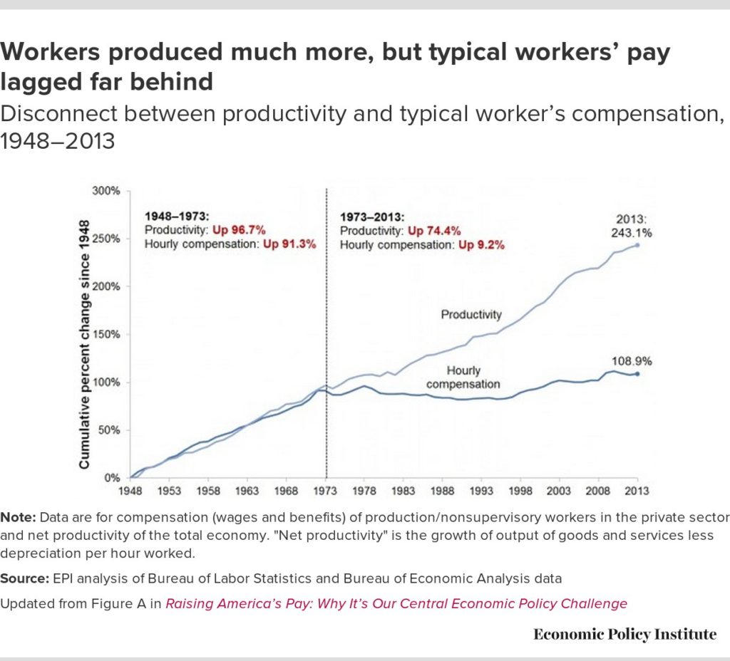
Productivity growth and real wages are closely linked. As productivity increases, workers can produce more output in the same or less amount of time, which enables employers to increase wages. However, as Figure 2 shows productivity in the US has been increasing but the typical worker’s compensation has not witnessed the same growth. 

Figure 2: Productivity and Typical Worker’s Compensation of Production/Nonsupervisory workers in the private sector between 1948 and 2013

Previous economic research emphasizes two explanations for these features. First, globalization has flooded the market with cheap goods from China and eroded domestic manufacturing wages in the process. Second, technology has brought about automation which has destroyed manufacturing jobs. 

However, as researchers from Kellogg Insight pointed out, US workers have struggled with wage stagnation for decades. Since the 1970s, growth in real wages, the value of the dollar paid to employees after being adjusted for inflation, has slowed compared to overall economic productivity. Furthermore, China did not begin to flood the market with cheap manufacturing exports until the mid-1990s, as seen in Figure 4. Lastly, job losses due to automation have primarily happened in the last 10 or 15 years. These three reasons suggest that import competition from China cannot be used as an explanation for stagnant wage growth and slowing economic growth. 

Despite the causes of these two economic factors, US-China trade relations are a source of concern for many, especially with escalating trade tensions under the Trump and now Biden administration. The interdependence of the US and Chinese economies has served as an “effective brake” on escalating strategic distrust. Both President Biden and President Xi are working to reduce the reliance each nation has on the other. 

Another source of stress stems from the US’ current accounts deficit, which is a measurement of a country’s trade where the value of the goods and services it imports exceeds the value of the goods and services which it exports. Because of this, the US typically borrows surplus savings from countries with current accounts surpluses and runs chronic current accounts deficits to attract more foreign capital. In 2020, China overtook Germany to become the world’s largest current account surplus. This was largely because the coronavirus crisis triggered higher demand for personal protective equipment and electronic devices, which boosted Chinese exports. China buys US treasury bonds using its current accounts surplus, and is the second largest US creditor, after Japan.

Many worry, however, that China will use its ownership of American debt as a bargaining chip to hold leverage over the US. However, the dollar is a widely-held and desirable asset in the global economy. While China has been the largest and second largest owner of US debt, the rest of the world (ROW) as well as individuals within the US still own the majority. For example, in August 2015, China reduced its holdings of US debt by roughly $180 billion, though this selloff did not significantly affect the US economy. Additionally, purchasing US debt enables China to manage the exchange rate of its currency, the renminbi. If China were to offload significant amounts of US debt, the exchange rate of the renminbi would rise and would make Chinese exports more expensive in foreign markets. 

Continued US debt financing worries economists who are concerned that a sudden stop in capital flows to the US could spark a domestic crisis; though this would only happen if demand for US debt from all financial actors, foreign and domestic, suddenly stopped.

Despite the trade deficit, there are significant benefits to the trade relationship between the US and China. According to a study by Oxford Economics, trade with China supports roughly 2.6 million jobs in the US across a range of industries, including jobs that Chinese companies have created in the US. The continued growth of the Chinese middle class, projected to exceed the population of the US by 2026, also serves as an enormous opportunity for US companies to expand their customer base, which will help bolster employment and economic growth. Furthermore, China’s role in the global supply chain improves the competitiveness of US businesses and lowers US inflation. 

Another factor that is often overlooked when tallying the balance of trade in the media is the contribution of US services exports to China. For example, trade data from the US Census Bureau only includes the trade of goods and not services. In 2019, the US exported $56.5 billion and imported $20.1 billion of services to China, a trade surplus of $36.4 billion. Chief US exports include capital products (22% of total exports), industrial supplies (22%), consumer goods (8%), and petroleum (7%). 

That Washington and the media place such a high emphasis on the trade deficit with China but not with Japan and the European Union with whom the U.S. also has trade deficits suggests that the trade deficit is used as a scapegoat for other areas of concern that they have with China. These main areas include alleged human rights abuses (such as in Xinjiang or Hong Kong), theft of intellectual property, and more.

Read More

·      Read this to learn more about trends in US real wages between 1979 and 2019. 

V. U.S.-China Trade War

In the leadup to the 2016 presidential election, Donald Trump used inflammatory comments to call out China, including saying that China was “raping” the U.S. with unfair trade practices and that the country was responsible for the “greatest theft in the history of the world.” Strategically building off of the growing backlash against globalization, Trump pledged to “cut a better deal with China which would help American businesses and workers compete” and accused China of manipulating its currency to make its exports more globally competitive. Steve Bannon, senior White House advisor, claimed that globalists gutted the American working classes and created a middle class in Asia. 

Once president, Trump renegotiated and revised trade agreements when US goals were not met. A key example of this is when he pulled out of the Transpacific Partnership (TPP), a multilateral trade agreement that would have created a single market for the US and the 11 countries that border the Pacific Ocean and would have maintained US trade dominance in Asia. Critics of the TPP argue that it would create wealth for multinational corporations rather than US workers.

Trump emphasized 1-on-1 bilateral negotiations with these Asian nations rather than joining the TPP, though he stressed that he would support future trade agreements if they were negotiated on a bilateral basis. This emphasis on bilateral negotiations demonstrates Trump’s belief that the global economy is a zero-sum conflict, where a gain for one party results in a corresponding loss for another party. Under this belief, multilateral negotiations result in allowing other countries to gain at the US’ expense. With bilateral agreements, the US would have greater leverage and be able to capture a greater share of the gains. 

Trump’s 2017 Trade Policy Agenda stated that the overarching objective of the trade policy was to “expand trade in a way that is freer and fairer for all Americans.” To achieve this, the Trump Administration would increase economic growth, promote job creation in the U.S., promote reciprocity with the U.S.’ trading partners, strengthen the manufacturing base and the ability to defend the U.S., and expand agricultural and service industry exports. In a not-so-subtle dig at China, the Agenda states that the U.S. should not turn a “blind eye” to unfair trade practices that disadvantage American workers, farmers, ranchers, and businesses in global markets. Rather, Washington should act as “aggressively as needed to discourage” unfair trading practices and to encourage true market competition.  

The Trump Administration executed this last statement with the ramping up of U.S.-China trade tensions in the first half of 2018 and the beginning of the trade war in July of 2018. A more complete timeline of the trade war can be found starting in Section 8. The US triggered the trade war starting in February 2018 with tariffs on solar panels meant to target Chinese firms and by initiating a WTO case against China. Trump increased these moves a month later targeting steel and aluminum imports. The next two years saw the imposition of tariffs, retaliatory tariffs, along with WTO cases alleging unfair trade practices from both the US and China. 

VI. Effect of the Trade War on the US-China Trade Deficit

Tariffs are taxes paid on imported goods, previously used as a key source of government revenue but more recently used to shield certain industries from foreign competition.

Tariffs are generally paid through three sources.

1. Foreign companies exporting goods to the US.
2. Domestic companies importing goods from abroad or using imported inputs in their production processes.
3. American households as final consumers.

Despite Trump’s insistence that the $79 billion in tariffs were paid by foreign companies, multiple studies have found that this is not the case. One such study found that by December 2018, import tariffs were costing US consumers and the firms that import foreign goods an additional $3.2 billion per month in added tax costs and another $1.4 billion per month in deadweight welfare (efficiency) losses.

Despite President Trump’s claims that the trade deficit hindered US economic growth, real gross domestic product saw an overall decrease between 2017 and 2019, with growth rates increasing from 2.37% to 2.93% but then down to 2.16%. The trade balance is not the only factor contributing to US economic performance and growth, which includes factors like employment, productivity, age of population, and more. 

VII. Conclusion

There are a multitude of factors causing the US-China trade deficit, not limited to the US current accounts deficit, Chinese currency manipulation, the shift in the US away from manufacturing jobs and towards service jobs, the growth of the information technology (IT) sector in the US and increased automation, and China’s comparative advantage in manufacturing that allows it to produce inexpensive goods. Furthermore, there are significant benefits to the US-China trade relationship, including lower aggregate prices for US consumers, and the promotion of at least 2.6 million jobs in the US. While increased import competition from China has resulted in the loss of several million manufacturing jobs, hitting the South and Midwest especially hard, overall trade with China has resulted in net job creation. Many view the US-China trade deficit as a sign of decaying US global leadership.

VIII. Timeline of US-China trade relations

1950-1972: US trade embargo with China

 In late 1950, China intervened in the Korean War on the North Korean side. Anti-communist rhetoric and propaganda, fueled by the Cold War, contributed to the belief that China was an intrinsic threat to US national security, leading President Truman to retaliate by imposing a total trade embargo with China. At the time, bilateral trade was roughly $200 million annually. President Nixon ended the embargo in 1972 with the hopes that improved US-Sino relations would aid the US in the Cold War with the Soviet Union. 

October 25, 1971: China joins UN

 The PRC assumed the ROC’s place in the GA as well as its place as one of the five permanent members of the UN Security Council (UNSC). 

February 1972: President Nixon makes historic trip to China to meet Chairman Mao

Nixon and Mao signed the Shanghai Communique, setting the stage for improved US-Sino relations by allowing China and the US to discuss difficult issues, particularly the China-Taiwan issue. For the rest of the decade, however, the two countries made slow progress in the normalization of their relations. 

1973: First American business delegation visits China since the founding of the PRC

At the time, there was not much bilateral trade or investment because China did not have much to sell to the US and the Chinese did not want to buy from the Americans. The Chinese government was still wary of foreign influence and Chinese culture was not receptive to business with foreign companies, because they wanted to be self-reliant. 

January 1, 1979: President Carter grants China full diplomatic recognition

Bilateral trade skyrocketed, creating a US trade surplus. At the time, the only investment model available for foreign companies was to establish a joint venture with a Chinese partner, which brought about conflicts with intellectual property (IP) theft. 

1979: China and the US sign trade agreement 

The trade agreement enabled Chinese products to receive temporary most favored nation (MFN) tariff status in the US. This made trading with China more attractive by lowering tariffs on goods imported to the US. 

1980: Deng Xiaoping launches economic “reform and opening” in attempt to jumpstart China’s economy and improve standard of living

Deng expands access for foreign businesses in China and US, Japanese, and European investment flood China. China also joins the IMF and the World Bank. 

Late 1980s and early 1990s: Surge of US investment into the PRC

China relaxed rules on foreign investment, including reforms which gave foreign companies permission to set up wholly foreign-owned enterprises in certain sectors, making it easier and more attractive to invest in China. 

June 1989: Tiananmen Square protests

The crackdown on protesters in Beijing’s Tiananmen Square marked a turning point for US-China trade relations as investors question whether China is a healthy and stable market and as the US implemented economic and trade sanctions as punishment for Beijing’s human rights violation. US-China relations became a political argument, notably during the 1992 presidential election campaign when Democratic nominee Bill Clinton accused incumbent Republican George H. W. Bush of being “soft” on China, particularly in relation to human rights, as he resisted calls for punitive measures following the Tiananmen Square massacre.  

1997: Asian financial crisis

October 10, 2000: US-China Relations Act of 2000

President Clinton granted permanent Normal Trade Relations (NTR) to China. This decision paved the way for China to ascend to the WTO. It reduced both tariff and nontariff barriers and fully opened the service sector to increased foreign ownership, especially in financial services, telecommunications, and distribution. 

December 11, 2001: China enters the World Trade Organization (WTO)

After 15 years of negotiation, China finally gained accession to the WTO. It was a transformational moment in the global economy, marking the beginning of a new era of globalization. China’s trade with the world increased. The WTO is a global international organization that handles the rules of trade between nations to help producers of goods and services, exporters, and importers conduct business

 2006: China surpassed Mexico as the US’ second-biggest trading partner, after Canada

2007: Chinese financial markets officially open to foreign investors under WTO rules

 2008-2017: China signed free trade agreements with Association of Southeast Asian Nations (ASEAN) bloc and others

September 2008: China became the largest US foreign creditor

China surpassed Japan and owned around $600 billion in US debt. This marked a growing interdependence between the US and Chinese economies and concerns over US-China economic imbalances grew. 

August 2010: China surpassed Japan to become the world’s second-largest economy

November 2011: US pivot toward Asia

Secretary of State, Hillary Clinton called for increased investment (diplomatic, economic, strategic, etc.) in the Asia-Pacific region as a move to counter China’s growing clout. 

2015: China announced its Made in China 2025 plan

This was the first industrial policy to indicate that China was interested in and capable of capturing global market share in high-tech industries that had been traditionally dominated by Western companies. 

2015: IMF added the Chinese yuan to its list of reserve currencies

February 3, 2016: Trans-Pacific Partnership is signed

Twelve countries (including the US), covering 40% of the world economy, signed the Trans-Pacific Partnership under President Obama. The TPP is advertised by President Obama as a “new type of trade deal that puts American workers first” and would help the US compete with China. The deal eliminated more than 18,000 taxes that various countries put on Made in America products. It also promoted a free and open internet, prevented unfair laws that restrict the free flow of data and information, and included the strongest labor standards and environmental commitments in history. The agreement included a 2-year ratification period in which at least 6 signatory countries must approve the final text for the deal in order for it to be implemented. 

January 20, 2017: President Trump is sworn into office

He was known for having an “America first” economic platform and was skeptical of free trade norms. Trump felt that China was “ripping off” the US and taking advantage of free trade rules to the detriment of US firms operating in China. 

January 24, 2017: Trump withdrew the US from the TPP

May 2017: US Secretary of Commerce, Wilbur Ross, unveiled a 10-part agreement between Beijing and Washington to expand trade of products and services such as beef, poultry, and electronic payments. The agreement did not address more contentious trade issues including aluminum, car parts, and steel. 

February 4, 2018: TPP was signed without the US

February 7, 2018: US implements new tariffs

The “global safeguard tariff” levied a 30% tariff on all solar panel imports (except those from Canada) and a 20% tariff on washing machine imports. Solar panel imports were worth $8.5 billion and washing machine imports were worth 1.8 billion 

March 22, 2018: US filed WTO case against China

President Trump signed a memorandum filing a WTO case against China for their discriminatory licensing practices.

March 23, 2018: US put in place new steel tariffs

Following months of threats, President Trump announced major penalty tariffs of 25% on all steel imports (with the exception of Argentina, Australia, Brazil, and South Korea) and a 10% tariff on aluminum imports (with the exception of Argentina and Australia). President Trump claimed these imports “threaten national security” and target China’s alleged unfair trade practices. Steel imports were worth at least $60 billion.

April 2, 2018: China imposed retaliatory tariffs 

China’s tariffs ranged from 15 to 25% on 128 US products worth $3 billion. This stoked growing fears of a trade war between the two biggest economies in the world. 

April 3, 2018: US proposed new tariffs

The United States Trade Representative (USTR) released a proposed list of 1,334 products (worth $50 billion) from China that could be subject to a 25% tariff.

July 6, 2018: US-China trade war officially began as US implements first China-specific tariff

The Trump administration imposed new tariffs on $34 billion of Chinese goods. More than 800 Chinese products in the industrial and transport sector faced a 25% import tax. China retaliated by imposing a 25% tariff on 545 goods originating from the US, worth $34 billion, including agricultural products, automobiles, and aquatic products. 

August 3, 2018: China announced a second round of tariffs on US products

August 14, 2018: China filed a WTO claim against the US 

The claim focused on US tariffs on solar panels and alleged that the US tariffs damaged China’s trade interests. 

August 23, 2018: US and China implemented second round of tariffs and China filed a second WTO complaint against the US

China retaliated and imposed a 25% tariff on 333 goods, worth $16 billion. 

September 24, 2018: US and China implemented third round of tariffs

October 4, 2018: Vice President Mike Pence delivered a critical speech against Beijing

Pence accused China of predatory economic practices, military aggression against the US, and of trying to undermine President Trump and harm his chances of winning re-election. Pence stated that the US will prioritize competition over cooperation by using tariffs to combat “economic aggression”

December 2, 2018: US and China agreed to a temporary truce 

The truce aimed to de-escalate trade tensions, following a working dinner at the G20 Summit in Argentina. Both the US and China agreed to refrain from increasing tariffs or imposing new tariffs for 90 days as the two negotiated for a larger agreement. 

December 14, 2018: China temporarily lowered tariffs on US automobiles for three months.

US auto imports are subjected to China’s standard 15% tariff rate on foreign autos. The suspension of additional tariffs is extended on March 31, 2019. 

April 1, 2019: China banned all strains of fentanyl

Chinese fentanyl production and distribution had been a source of tension in bilateral relations because of the opioid crisis in the US. 

April 10, 2019: US and China agreed to establish trade deal enforcement officers to monitor the enforcement of the trade deal, which has not yet been finalized

May 10, 2019: Trade war intensified

The US increased tariffs on $200 billion worth of Chinese goods from 10% to 25%. President Trump stated that he believes the high costs imposed by the tariffs will force China to make a deal favorable to the US.

May 13, 2019: China retaliated and announced it will increase tariffs on $60 billion worth of US goods starting June 1

May 16, 2019: US Department of Commerce announced the addition of Huawei Technologies Co. Ltd and its affiliates on its “entity list,” which effectively banned US companies from selling to the Chinese telecommunications company without US government approval. 

 June 2, 2019: China issued a white paper on US-China economic relations found here. 

The paper denounced US unilateral and protectionist measures, criticized its backtracking on Sino-US trade talks, and demonstrated China’s stance on trade consultations and the pursuit of reasonable solutions. 

June 21, 2019: US Department of Commerce added 5 more Chinese companies to its “entity list”

Sugon, the Wuxi Jiangnan Institute of Computing Technology, Higon, Chengdu Haiguang Integrated Circuit, and Chengdu Haiguang Microelectronics Technology were added to the list.

August 6, 2019: US Treasury labeled China as a currency manipulator 

The yuan sank to 7 against the US dollar in apparent retaliation to the new punitive tariffs threatened to apply on the remainder of Chinese imports. China denied the accusations. The US later dropped this designation days before signing the phase one trade deal.

August 23, 2019: China announced $75 billion in tariffs on US goods. 

September 1, 2019: US began implementing tariffs on more than $125 billion worth of Chinese imports. 

September 2, 2019: China lodged a WTO tariff case against the US

According to WTO rules, the US has 60 days to try to settle the latest dispute. 

October 11, 2019: President Trump announced that the US and China have reached a “Phase 1” agreement and that the US will delay a tariff increase. 

November 1, 2019: WTO stated that China can impose compensatory sanctions on US imports worth $3.6 billion for the US failure to abide by anti-dumping rules on Chinese products. 

January 15, 2020: US and China signed the ‘Phase 1’ trade deal, easing 18-month trade tensions

The trade deal relaxed some US tariffs on Chinese imports and committed China to buying an additional $200 billion worth of American goods (including agricultural products and cars) over 2 years, though the majority of tariffs remain in place

January 20, 2021: President Biden is sworn into office and planned to remain tough on China

Cabinet members signalled that Biden plans to take a multilateral approach by enlisting the support of Western allies to maximize Washington’s leverage on Beijing.